
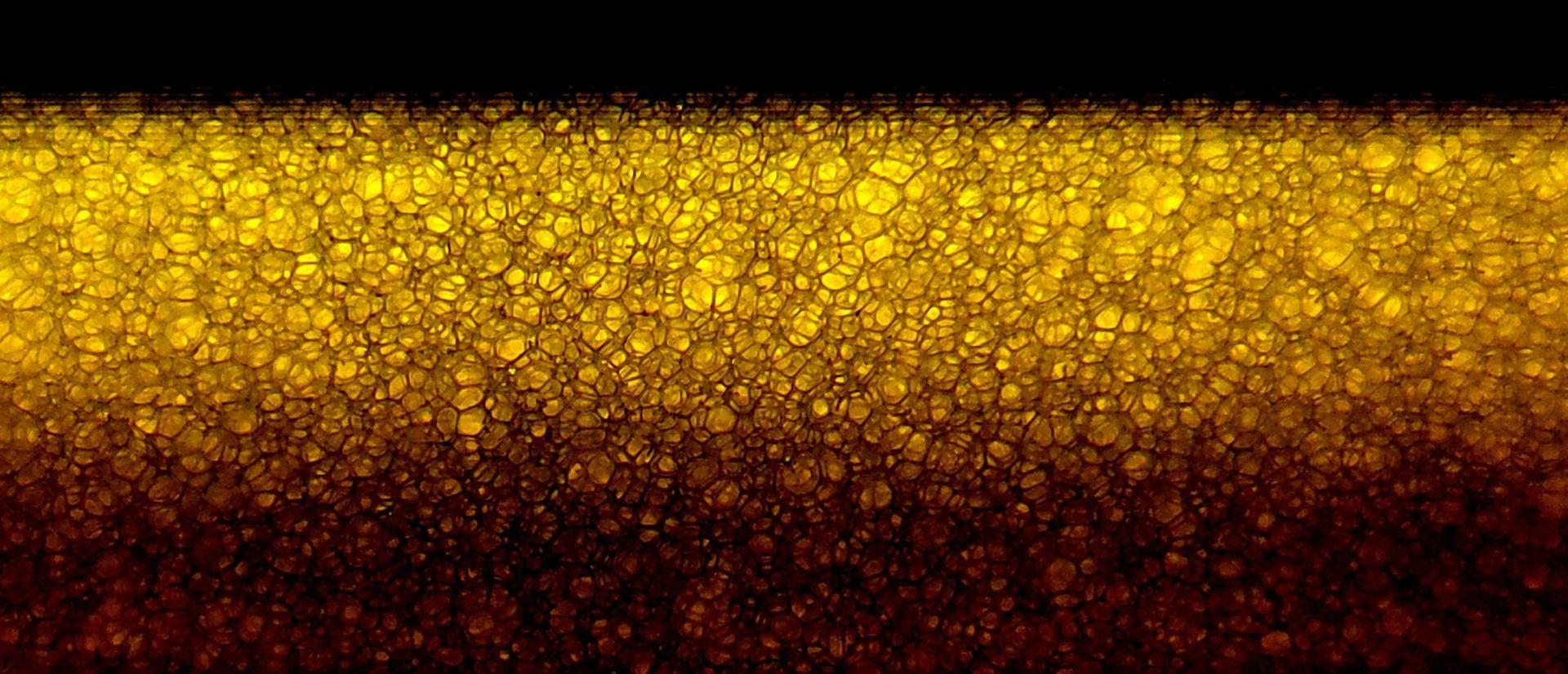
Summary
A classical computer vision routine was developed to measure surface texture on a homemade sourdough bread, using 31 photographs taken with a mobile phone under three deliberately different imaging conditions.
Four findings:
- A repeatable measurement is achievable with non-specialized consumer equipment — 3.2% coefficient of variation on surface roughness, adequate for quantitative work.
- Lighting accounts for 94% of measurement variance; part fixturing for 0%, confirmed independently by two different metrics.
- The material has no natural pore/surface threshold. Any thresholded "porosity" figure from this bread is an artifact of the threshold chosen, not a property of the bread.
- A metric with no free parameters matches a three-parameter pipeline on repeatability, and should replace it.
Five iterations of imaging setup preceded the first line of inspection code. That ratio was not a detour: it is the finding.
1. Objective
The bread's surface texture is currently assessed by a subjective appearance score (0–3). The question for this study: can an objective, repeatable, quantitative texture measurement be established using available equipment?
Secondary question: how much of the measurement variation is attributable to lighting versus part placement, since that determines where capital should go in any future automated system.
2. Phase 1 — Imaging setup: five iterations
Iteration 1 — Underexposed
| Mean | Std | 5th–95th percentile | Clipping |
|---|---|---|---|
| 77.2 | 40.7 | 38–179 | 0.00% / 0.00% |
No clipping, which is the condition that cannot be corrected later. But the mean sat at 77 against a scale midpoint of 127.5, using only 55% of the available dynamic range. Photon shot noise scales with the square root of signal, so an underexposed image is a noisier image at the same ISO — and brightening it afterwards amplifies noise along with signal.
Iteration 2 — Correct mean, collapsed contrast
| Iteration 1 | Iteration 2 | |
|---|---|---|
| Mean | 77.2 | 154.4 |
| Std | 40.7 | 11.1 |
| 5th–95th range | 141 wide | 33 wide |
| Dynamic range used | 55% | 13% |
Exposure was raised to hit a target mean of 110–140. The mean was achieved exactly and contrast fell by a factor of nearly four.
This was a failure of the instruction, not the execution. A single-metric target was set — raise the mean — and the metric that actually matters for inspection was not constrained. Mean intensity is where the signal sits on the scale; contrast is the signal.
An exposure increase alone multiplies pixel values and stretches the histogram; with no clipping, standard deviation should have risen to roughly 80. That it fell to 11 indicated a second variable had changed: either framing onto a more uniform region, flatter lighting, or the phone's HDR tone mapping engaging and compressing dynamic range.
Iteration 3 — Contrasting background
| Mean | Std | 5th–95th | Separation / noise |
|---|---|---|---|
| 87.8 | 59.8 | 22–180 | 6.71 |
Otsu threshold 94; dark region 37.3 ± 11.3, light region 152.5 ± 23.0, separation 115.2 intensity units.
A separation-to-noise ratio of 6.71 is excellent — but it was measuring object against backdrop, which is the easy problem and not the inspection task. Inspection requires separating features from the object's own surface.
Iteration 4 — The two-stage check revealed the real problem
Masking the object and re-thresholding within it:
| Value | |
|---|---|
| Threshold | 39 |
| Features | 29.4 ± 5.8 (56.8% of object) |
| Surface | 48.3 ± 9.6 |
| Separation / noise | 2.45 |
The ratio of 2.45 appeared acceptable. The 56.8% split was the real signal.
Features should be a small minority of a surface. A near-even split means Otsu found one broad population and bisected it — and bisecting a normal distribution yields a separation-to-noise ratio of approximately 2.7 by construction. The 2.45 was measuring the width of a single population, not a gap between two.
The underlying cause was dynamic range theft: the bright backdrop (152) forced the exposure down, leaving the object (surface 48, features 29) in the darkest fifth of the sensor range with only 19 intensity units of separation.
The contrasting background that made object isolation trivial was actively preventing surface inspection.
Iteration 5 — Fill the frame, expose for the object
| Mean | Std | Clipping |
|---|---|---|
| 154.4 | 18.2 | 0.00% / 0.00% |
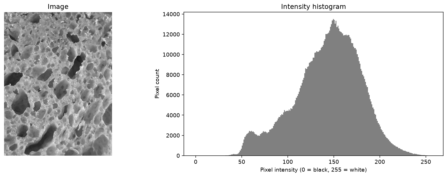
Percentile analysis against the surface median of 156:
| Darkest fraction | Below | Gap from median | Normal would predict |
|---|---|---|---|
| 1% | 110 | 46 | 114 |
| 2% | 115 | 41 | 119 |
| 5% | 122 | 34 | 126 |
| 10% | 130 | 26 | 133 |
| 20% | 139 | 17 | 141 |
| 30% | 146 | 10 | 147 |
The observed tail ran consistently 2–4 units darker than noise alone would produce, with the deviation widening toward the extreme — the signature of a small dark population pulling the tail down.
Suggestive but not decisive. A 4-unit deviation cannot distinguish real sparse features from slightly skewed noise.
The spatial coherence test settled it
Noise is spatially random; structure is spatially clustered. That difference requires no statistical assumption.
| Threshold | Regions | Dark pixels | Median region | Largest | Regions ≥10 px | Dark pixels in regions ≥10 px |
|---|---|---|---|---|---|---|
| 110 (1%) | 382 | 10,515 | 3 px | 1,757 px | 97 | 93% |
| 115 (2%) | 541 | 21,439 | 3 px | 3,765 px | 138 | 95% |
| 122 (5%) | 814 | 50,067 | 3 px | 17,724 px | 185 | 97% |
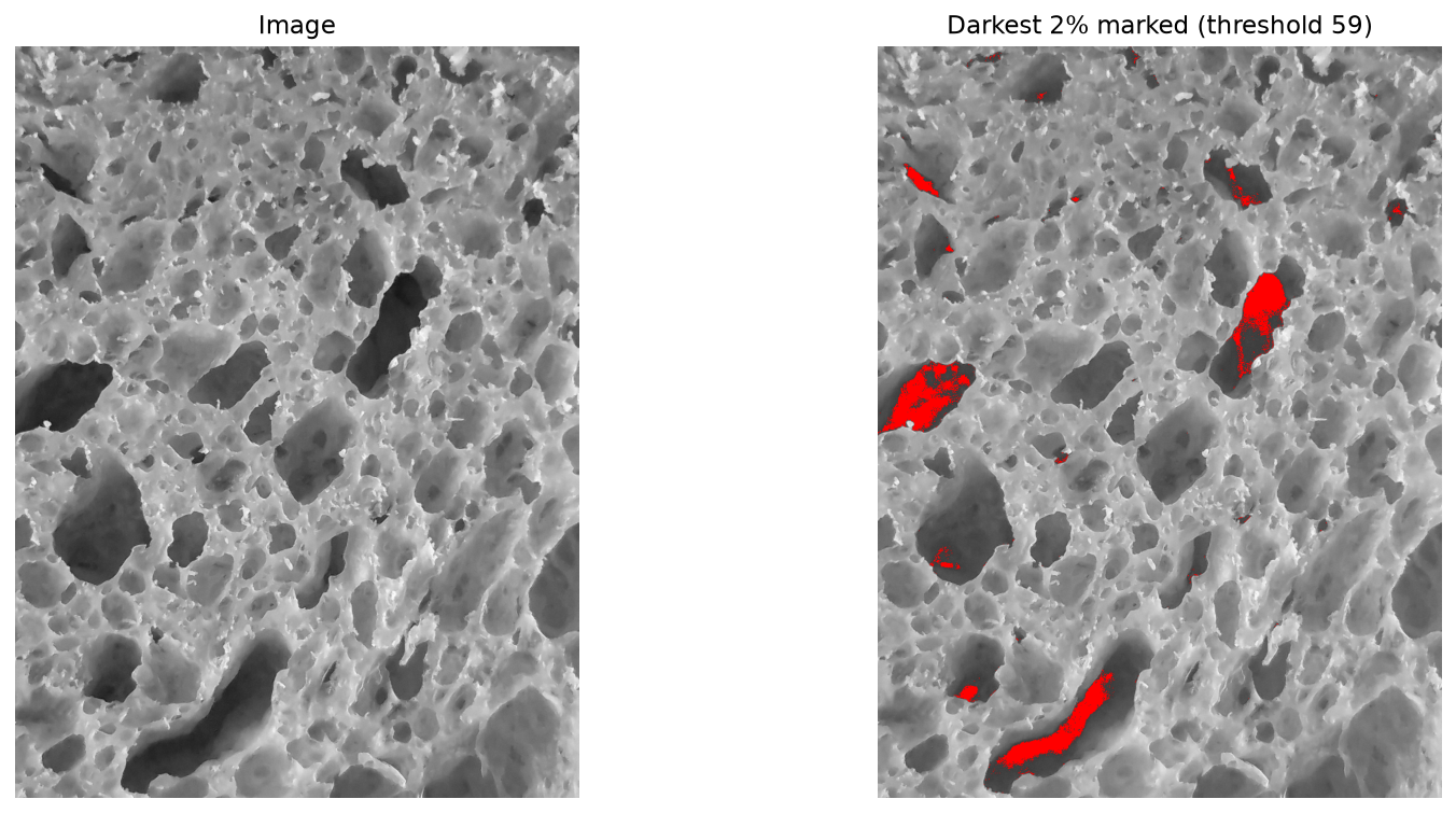
93–97% of dark pixels sat in connected regions of 10 pixels or more. Real, coherent structure.
The region-size distribution also revealed a clean split: of 382 regions at the 1% threshold, only 97 exceeded 10 pixels, and the remaining 285 one-to-three-pixel specks accounted for just 7% of dark pixels. This gave an evidence-based minimum area filter rather than a guessed one.
One warning signal was noted and deferred: the largest region grew from 1,757 to 17,724 pixels as the threshold loosened, reaching 35% of all detected area at the 5% threshold. Candidate causes were vignetting, edge shadow, or feature merging.
Setup locked
Resolution          92.2 px/mm (full resolution)
1 pixel             10.8 µm
3-pixel limit       33 µm
Region of interest  1600 px central crop ≈ 17.4 × 17.4 mm = 301 mm²
Vignetting          11.7 units centre-to-corner — removed by central crop
Minimum area        0.013 mm² = 111 px = 0.13 mm equivalent diameter
Exposure            fixed, HDR disabled
A critical scale correction was required. The minimum-area threshold of 10 px had been derived on a downscaled image at 27.7 px/mm, then converted using the full-resolution 92.2 px/mm — an eleven-fold error in area. The fix was structural: define every threshold in physical units (mm²) and compute the pixel equivalent, making the error impossible to repeat.
3. Phase 2 — Capture protocol
Three sets, to permit variance decomposition:
| Set | Images | Protocol | Isolates |
|---|---|---|---|
| Controlled | 11 | nothing touched between frames | imaging chain alone |
| Replaced | 10 | object lifted and replaced each frame | imaging + fixturing |
| Degraded | 10 | poor lighting angle, tilt, harsh light, varied distance, one defocused | imaging + lighting |
Separate shutter presses throughout, never burst mode — burst frames share one exposure decision and would have understated repeatability by measuring sensor read noise.
Illumination consistency
| Set | Mean intensity | Std | CV | Max clipping |
|---|---|---|---|---|
| Controlled | 144.3 | 2.19 | 1.5% | 0.00% |
| Replaced | 143.9 | 2.03 | 1.4% | 0.00% |
| Degraded | 137.5 | 10.41 | 7.6% | 0.06% |
Removing and replacing the object changed illumination statistics not at all — physically expected, since the lamps and camera never moved. The degraded set showed 4.8× the variation and the first clipping observed in the study.
4. Phase 3 — Pipeline and parameter selection
Five stages: Gaussian blur → adaptive threshold → morphological open and close → connected components → area filter.
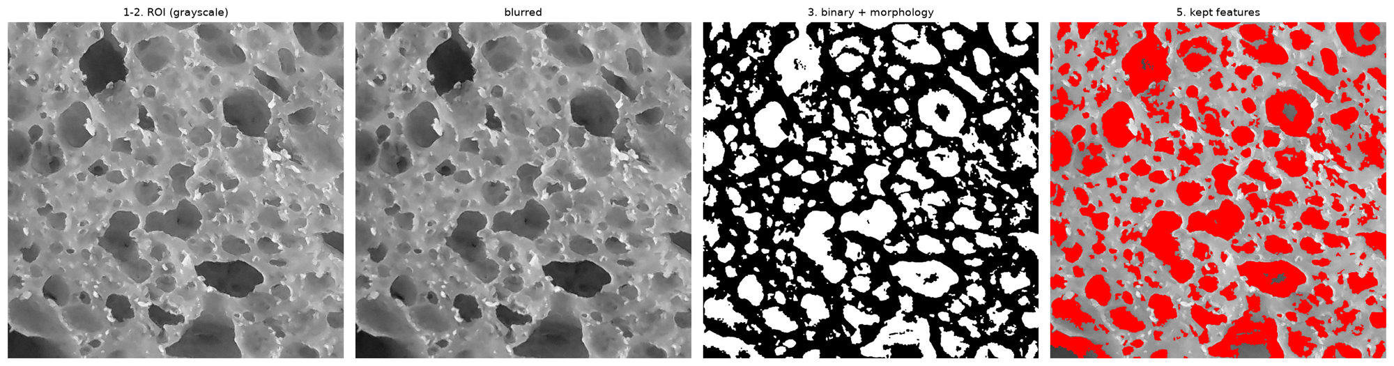
Block size sweep
| Block | Physical size | Count | Area (mm²) |
|---|---|---|---|
| 51 | 0.55 mm | 614 | 41.59 |
| 101 | 1.10 mm | 498 | 84.66 |
| 151 | 1.64 mm | 377 | 106.35 |
| 251 | 2.72 mm | 258 | 122.29 |
| 261 | 2.83 mm | 253 | 122.99 |
| 271 | 2.94 mm | 249 | 123.42 |
| 401 | 4.35 mm | 207 | 123.93 |
Detected area plateaus from block 251 upward. Count never converges. The first divergence between the two metrics, and an early signal that count was not a measurement.
Block 271 was selected — in the plateau region, and roughly six times the largest feature dimension.
Adaptive versus global thresholding
| Method | Count | Area (mm²) |
|---|---|---|
| Adaptive | 249 | 123.42 |
| Otsu (global) | 149 | 104.65 |
Adaptive was retained on principle, given the measured 11.7-unit vignetting. Unplanned confirmation arrived later from the data itself — see Section 6.
5. Phase 4 — Repeatability and variance decomposition
Measured coefficients of variation
| Metric | Controlled | Replaced | Degraded | Parameters |
|---|---|---|---|---|
| roughness_std | 3.2% | 3.2% | 13.4% | none |
| total_area_mm² | 3.0% | 2.6% | 12.4% | 3 |
| roughness_iqr | 6.0% | 7.5% | 12.5% | none |
| dark_depth_p5 | 5.9% | 7.8% | 11.1% | none |
| dark_depth_p1 | 6.2% | 6.4% | 9.6% | none |
| mean_area_mm² | 12.8% | 9.8% | 26.1% | 3 |
| count | 12.7% | 9.1% | 27.7% | 3 |
| skew | 32.8% | 52.7% | 107.7% | none |
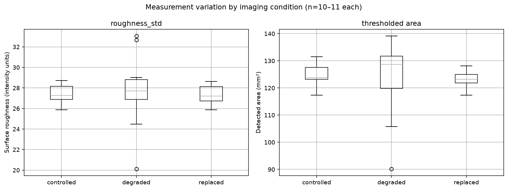
Decomposition
σ²_controlled = σ²_imaging
σ²_replaced   = σ²_imaging + σ²_fixturing
σ²_degraded   = σ²_imaging + σ²_lighting
| Source | total_area_mm² | roughness_std |
|---|---|---|
| Imaging chain | 3.02% CV — 6.0% of variance | 3.20% CV — 5.7% |
| Fixturing | 0.00% CV — 0.0% | 0.00% CV — 0.0% |
| Lighting degradation | 11.99% CV — 94.0% | 13.01% CV — 94.3% |
Two independent metrics agree to within 0.3 percentage points. The attribution is a property of the imaging, not of the measurement approach.
σ²_replaced − σ²_controlled is negative for the area metric (2.64² − 3.02²), reported as zero per gauge R&R convention. The correct reading is that fixturing lies below the detection limit of an 11-frame study, not that it is exactly zero.
Why count failed, with the mechanism
The degraded set shows it directly:
| Controlled | Degraded | Change | |
|---|---|---|---|
| count | 193.5 | 180.4 | −6.8% |
| mean_area_mm² | 0.655 | 0.730 | +11.5% |
| total_area_mm² | 124.9 | 123.3 | −1.3% |
Fewer features, each larger, the same total area. Shadows are connecting adjacent features into single regions. Count is topologically fragile — one bright pixel bridging two features changes it by one while barely moving the area. Connectivity is what noise perturbs first.
6. Phase 5 — The threshold finding
Sweeping the adaptive threshold offset:
| C | Count | Area (mm²) | Area fraction |
|---|---|---|---|
| 2 | 228 | 143.27 | 47.6% |
| 5 | 249 | 123.42 | 41.0% |
| 10 | 253 | 90.40 | 30.0% |
| 20 | 163 | 40.52 | 13.5% |
| 30 | 107 | 15.99 | 5.3% |
| 40 | 59 | 4.72 | 1.6% |
| 50 | 12 | 0.88 | 0.3% |
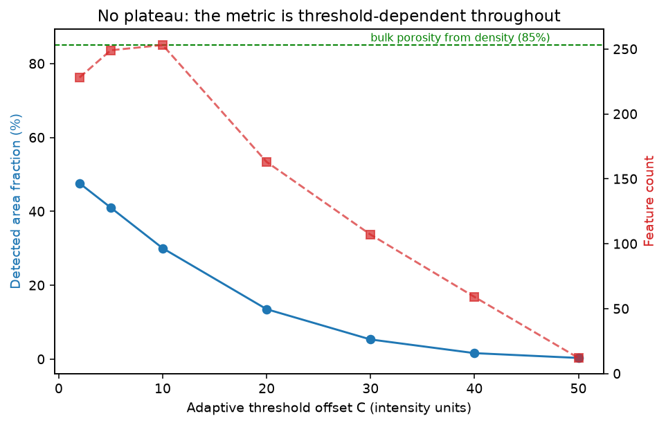
No plateau at any value. A smooth monotonic decay from 47.6% to 0.3%.
A plateau appears where two populations are separated by a gap. Its absence, combined with the earlier coherence result showing 93–97% of dark pixels in coherent regions, gives a consistent picture: the dark regions are real structure at every threshold, but no scale separates "pore" from "slightly recessed surface."
This is physically correct for a surfactant-foamed fibre composite. The surface is not a smooth plate with discrete holes; it is an open cellular structure in which cell walls, partial cells, inter-fibre voids and surface relief form a continuous distribution of depths. The material has no natural boundary for an algorithm to find.
The Iteration 4 result — a 56.8% split on a unimodal within-object histogram — had been pointing at this from the start.
Validation against an independent measurement
Bread density        ~214 kg/m³
Skeletal density     ~950 kg/m³  (flour)
Bulk porosity        1 − 214/950 = 77%
Detected at surface  41.5%        (301 mm² ROI, 124.9 mm² detected)
Detecting roughly half the porosity present is coherent: the balance lies below the 0.13 mm detection limit or beneath the surface skin.
This cross-check is a stronger validity test than any software diagnostic, and it was available only because an independent physical measurement already existed.
Consequence
"Pore area fraction" is not a well-defined measurement for this material. At C = 5 the answer is 41%; at C = 30 it is 5.3%. Both are equally defensible, which means neither is a property of the bread.
Any porosity figure previously quoted from image analysis of these bread slices was threshold-dependent and is unlikely to be comparable to anything.
Threshold-free alternative
roughness_std — the standard deviation of the intensity residual after flat-field correction — achieves 3.2% CV against the thresholded metric's 3.0%. F = 1.14 at 10 and 10 degrees of freedom: a tie.
Selected on engineering grounds: no parameters to defend, no topological fragility, physically interpretable as RMS surface relief, and identical repeatability with and without part replacement (3.2% / 3.2%) where every other metric degraded. That last property means it requires less fixturing precision than the thresholded approach.
Its one cost: marginally greater lighting sensitivity (13.4% vs 12.4% on the degraded set), since relief amplitude as seen by a camera is directly a function of illumination angle.
7. An unplanned robustness test
The per-frame data from the controlled set contained an accidental experiment:
| Illumination (roi_mean) | Measured area (mm²) | |
|---|---|---|
Frame 20261030_122046 |
153.6 | 125.4 |
| All other frames | 143.0–149.0 | 117.3–131.6 |
One frame received 5–7% more illumination than every other, and its area measurement landed almost exactly on the set mean (124.9 mm²).
Adaptive thresholding absorbed the excursion with no measurable effect. A global threshold would have shifted. This is direct evidence from the study's own data for the adaptive-over-global choice made on principle in Phase 3.
8. Findings
1. A quantitative, repeatable surface measurement is achievable with consumer equipment. 3.2% CV using a mobile phone, two lamps and open-source software. Adequate for quantitative work by conventional gauge R&R standards (under 5%).
2. Lighting accounts for 94% of controllable measurement variance; fixturing for 0%. Confirmed independently by two metrics. Capital in any automated system should go to illumination, optics and exposure control ahead of jigs and ahead of software.
3. Degraded imaging produces four times the variance and cannot be recovered by tuning. Parameter sweeps traded one failure mode for another; none restored controlled-set performance. The information was destroyed at capture.
4. Report area, never count. 3.0% versus 12.7% CV, with the connectivity mechanism identified and quantified.
5. The bread surface has no natural pore threshold. Thresholded "porosity" figures are parameter artifacts. Either define the measurement operationally and publish the procedure, or use a threshold-free metric.
6. A zero-parameter metric matches a three-parameter pipeline. roughness_std should replace thresholded area as the primary measurement.
7. An objective replacement for the subjective appearance score now exists. Whether it tracks anything the appearance score was capturing is the next question.
9. What went wrong, and what it taught
Five documented errors, each with a transferable lesson.
| Error | Lesson |
|---|---|
| Exposure raised to a target mean; contrast collapsed 4× | Optimise the metric that matters, not a proxy. Mean intensity is where the signal sits; contrast is the signal. |
| Separation ratio of 2.45 accepted on a 56.8% split | A balanced split on a sparse-feature problem is itself the failure signal. Bisecting one population yields ≈2.7 by construction. |
| A contrasting background chosen for object isolation | It stole the dynamic range. The right choice for one stage was the wrong choice for the next. |
| Minimum area derived at one resolution, converted at another | Define thresholds in physical units. An 11-fold error, structurally preventable. |
| Three sets captured as contiguous blocks | Randomise capture order across conditions. The same discipline as randomising run order in a designed experiment. |
The two most useful diagnostics in the study were not statistical tests:
Spatial coherence — noise is scattered, structure is clustered. Connected-component size distribution settles signal-versus-noise in one step, with no distributional assumption.
The plateau test — sweep the principal parameter and look for convergence. No plateau means the reported value is a property of the parameter rather than of the object.
10. Limitations
Sample size. 10–11 frames per set. Standard error on a standard deviation at n = 10 is approximately σ/4.2, giving roughly ±25% relative uncertainty on each CV figure. Differences below about 1 percentage point are not resolvable.
Possible temporal drift. Measured area correlated with capture order at r = −0.507 across 11 frames. Critical r at n = 11 is 0.602, so p ≈ 0.11 — suggestive, not significant. Illumination showed no matching trend, so lamp warming is excluded as a cause. The first six frames averaged 127.0 mm² against 122.2 mm² for the last five.
Capture order not randomised. Had the drift been real, it would be confounded with the set difference. The degraded effect is approximately 4× too large to be explained by a 4% trend, so the principal conclusion is unaffected.
Single object. All 31 frames are of one bread. Between-bread variation is entirely unmeasured.
Fixturing result is metric-specific. The 0% contribution applies to a global statistic computed over a region of interest, which is inherently tolerant of small translations and rotations. A metric requiring feature-level correspondence — dimensional measurement, registration, position verification — would show a substantial fixturing contribution.
Validity unproven. Precision is demonstrated; whether roughness_std tracks any physical property of the bread is untested.
Skeletal density assumed. The 950 kg/m³ figure used in the porosity cross-check is a literature value for flour, not a measurement on this material.
11. Next steps
Establish validity. Photograph 10–15 bread slices spanning the available density range (180–308 kg/m³) and test whether roughness_std correlates with measured density. If it does, the result is an image-based proxy for a property currently requiring a cut and weighed specimen. If it does not, the metric is repeatable and meaningless. Approximately one hour's work.
Test against the appearance score. The same images, correlated against the existing subjective appearance rating. Agreement would validate the score and offer to replace it; disagreement would indicate that appearance captures something the texture metric does not.
Randomise and extend the repeatability study. Interleave the three sets and increase to 20 frames each, which would resolve whether the observed drift is real and halve the uncertainty on the CV figures.
Investigate the large-region growth. The largest connected region reaching 35% of detected area at the 5% threshold remains unexplained — vignetting, edge shadow or feature merging. Relevant if the thresholded metric is retained for any purpose.
Measure skeletal density to put the porosity cross-check on a measured rather than literature basis.