

1. The governing idea
A model that knows what it doesn't know can tell you what to do next.
Every model built before produced point predictions, useful for understanding a process, useless for deciding which experiment to run. A prediction of 58 MPa gives no basis for choosing between two candidate formulations. A prediction of 58 ± 2 against 55 ± 12 does, and the second may well be the better experiment precisely because nobody knows what it does.
Calibrated uncertainty is what converts a predictive model into an experimental planning tool. That is the whole of Bayesian optimisation.
Uncertainty also tells you when a programme cannot be optimised at all. If measurement noise consumes most of the variance, an optimiser will propose candidates with complete confidence, derived entirely from noise.
2. Glossary
Models with uncertainty
Gaussian process (GP): A model that returns a predicted value and a calibrated uncertainty for every point. It assumes similar inputs give similar outputs: confident near observed data, reverting toward the mean with widening uncertainty far from it. Practical meaning: the right tool whenever the next action depends on knowing where the model is ignorant — optimisation, experimental design, active learning. Also well suited to small datasets, where it degrades gracefully rather than overfitting.
Kernel: The function encoding what kind of response surface is expected. Determines how quickly the model assumes the output changes as inputs change. Practical meaning: the kernel is where domain knowledge enters a GP. Choosing it is a modelling decision, not a default.
Matérn kernel (ν = 2.5): Assumes the response is smooth but not infinitely so. Practical meaning: the standard choice for physical systems. The RBF default assumes infinite differentiability, which is unrealistically smooth for real materials and produces overconfident predictions.
Length scale: How far an input must move before the output changes appreciably. Fitted per dimension. Practical meaning: short length scale = the variable matters; long = it does not. A free sensitivity analysis produced as a by-product of fitting.
Automatic Relevance Determination (ARD): Giving each input its own length scale, so the model learns which variables are informative. Practical meaning: variable importance, obtained without a separate analysis. Check it against known physics as a plausibility test.
WhiteKernel: A noise term estimating measurement error. Practical meaning: the GP's own estimate of the noise floor, inferred from the data without replicates. Valuable where repeat measurements are unavailable. Compare it against measured repeatability where both exist.
Optimisation
Bayesian optimisation (BO): Fit a surrogate model with uncertainty, use it to choose the next experiment, run it, refit, repeat. Practical meaning: a structured alternative to intuition-led or grid-based experimentation. Known in materials science as active learning, self-driving labs, or autonomous experimentation.
Surrogate model: A cheap statistical stand-in for an expensive experiment or simulation. Practical meaning: makes it feasible to evaluate thousands of candidate formulations computationally before committing to a handful in the lab.
Acquisition function: The rule converting a model's predictions and uncertainties into a decision about what to try next.
Expected Improvement (EI): The most common acquisition function: the expected amount by which a candidate beats the current best. Practical meaning: balances exploitation (go where the prediction is high) against exploration (go where uncertainty is high) without requiring a tuning parameter. The balance emerges from asking the right question.
Exploration vs exploitation: Pure exploitation polishes a local optimum and never finds anything better. Pure exploration wanders into regions nobody cares about. Practical meaning: the central trade-off in sequential experimentation, and the reason intuition-led campaigns often stall — experienced developers tend to over-exploit near what already works.
Trials to target: The number of experiments needed to reach a defined performance threshold. Practical meaning: the only optimisation metric that converts directly into money and calendar time. Report the median and the worst case.
Pruning (optuna.TrialPruned): Declaring a candidate infeasible so the optimiser disregards it. Practical meaning: the correct way to encode constraints. Cleaner than returning a large penalty, which distorts the search surface.
Experimental design
Statistical power: The probability of detecting an effect that genuinely exists. Conventionally 0.80. Practical meaning: at 80% power, a correctly designed experiment still misses a real effect one time in five.
Minimum detectable difference (δ): The smallest effect an experiment can reliably detect. Practical meaning: a commercial decision, not a statistical one. It must be set by what a customer, specifier, or process would notice — not by what feels precise.
Underpowered: Having too few samples to detect effects of the size expected. Practical meaning: an underpowered experiment cannot produce a usable negative result. "No effect found" is indistinguishable from "effect too small to see," and the money is spent either way.
Staged design: Splitting a campaign into sequential stages, each informing the next. Practical meaning: usually superior to a full factorial when effect sizes differ by an order of magnitude. Replicate where the uncertainty is, not uniformly.
3. Principles
3.1 Use a model with uncertainty when the next action depends on the answer
Point predictions suffice for understanding. Decisions about what to do next require knowing the model's confidence.
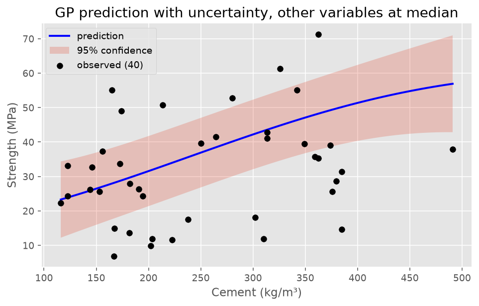
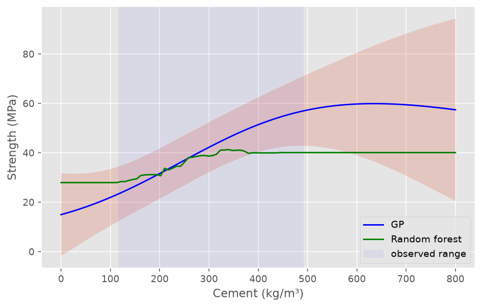
The contrast that makes this concrete: outside its training range, a random forest predicts a flat constant with no warning. A Gaussian process reverts toward the mean with a visibly widening band. Since optimisers push toward unexplored regions by design, only the second is safe to optimise against.
3.2 At small n, feature selection is forced, not optional
With 40 samples and six features, a GP cannot identify length scales for all dimensions — several slide to their optimiser bounds and the fit becomes unstable.
Reducing to two physics-derived features improved both accuracy (6.28 → 5.83 MPa) and stability (fold-to-fold σ 2.01 → 1.32).
Stability matters as much as accuracy. A model with low fold variance behaves consistently whichever samples it trains on; a high-variance model is at the mercy of which rows landed in training.
Rule of thumb: a GP needs roughly 10–15 samples per dimension to identify length scales reliably. Below that, strip features until the pinning stops.
3.3 A pinned length scale is a convergence failure, not a finding
A length scale orders of magnitude larger than its neighbours, sitting at the optimiser's bound, means the model could not determine the value — not that the variable is irrelevant.
Two causes:
- The variable acts through an interaction or ratio rather than alone
- Insufficient data to resolve that dimension
Always set explicit bounds (length_scale_bounds=(1e-2, 1e3)) so pinning is visible rather than disappearing into a default of 100,000.
3.4 Encoding changes conclusions
Water as a raw mass produced a length scale of 27,660 — effectively excluded. As a water-to-binder ratio, it became the second most important variable.
Identical information, different encoding, opposite conclusion. A model given raw masses would have reported that water does not affect concrete strength.
Encoding physical relationships is a domain-expertise task. No amount of algorithm selection substitutes for it, and this is the clearest demonstration of where a materials engineer outperforms a data scientist on the same dataset.
3.5 One split is one draw — this applies to optimisation too
A single train-test comparison showed the raw-water model beating the ratio model. Under repeated cross-validation the ordering reversed.
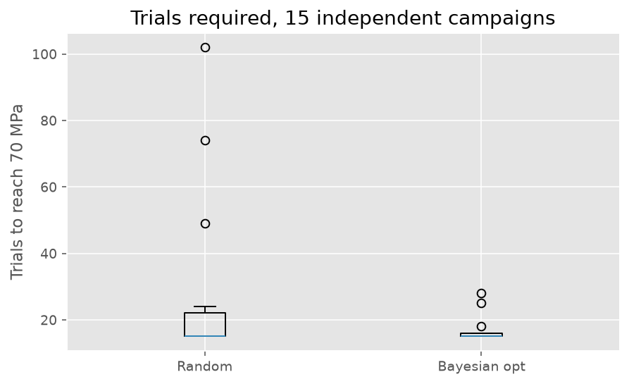
The same logic governs optimisation campaigns. Run 15 or more seeds and report the distribution. A single simulated campaign tells you almost nothing, because the starting sample dominates the result.
3.6 Report the worst case, not only the median
| Strategy | Median | Range | Failures |
|---|---|---|---|
| Random | 76 | 8–201 | 2 of 15 |
| Bayesian opt | 15 | 8–30 | 0 of 15 |
The median is the headline. The tail is what programme managers care about. A campaign that usually takes 20 trials and occasionally takes 200 cannot be scheduled or budgeted; one that never exceeds 30 can.
Predictability is a distinct benefit from speed, and it is frequently the more persuasive one.
3.7 Make the target difficult enough to discriminate
An initial comparison returned a median of exactly 15 trials for both strategies — the number of random initial samples. The target was being hit by the starting draw before either method made a choice.
If the median equals n_init, no strategy was tested. Choose a target that only 1–3% of the candidate space satisfies, and reduce the number of initial samples.
3.8 An optimum on a boundary is a diagnostic
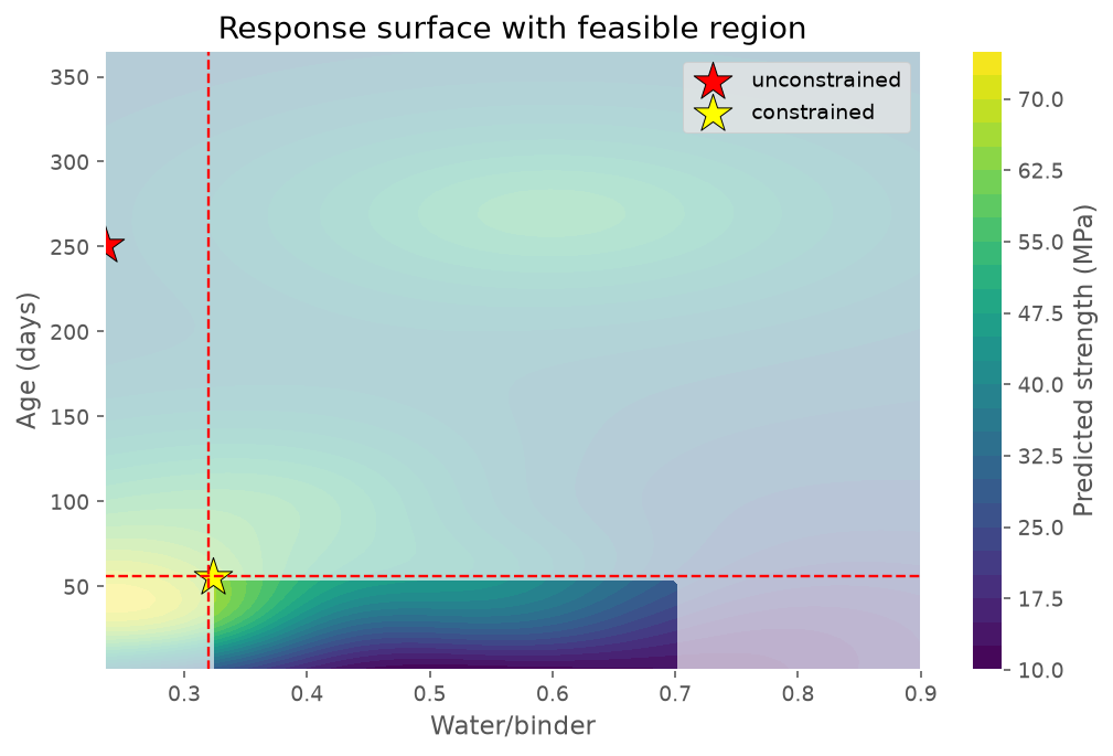
Fifth and sixth occurrences of this pattern in the curriculum. An optimiser pressed against a limit means the objective function is missing a constraint that exists in reality.
Two cases requiring opposite responses:
| Situation | Meaning | Response |
|---|---|---|
| Pinned with no constraint present | Missing constraint; result is an artefact | Add the constraint |
| Pinned on a real constraint | Constraint is binding | Nothing — this is the answer |
In the second case, the optimum sits on the constraint because the response is monotonic within the feasible region. Further gain requires moving the constraint, not searching harder.
3.9 Constraints have a measurable cost — quantify it
| Constraints | Achievable | Cost |
|---|---|---|
| None | 81.0 MPa | — |
| Placeability only | 70.1 MPa | −10.9 |
| Age limit only | 72.4 MPa | −8.6 |
| Both | 61.3 MPa | −19.7 |
Nobody can sensibly challenge a constraint until they know what it costs. Attribute them individually — if roughly additive, they act on independent axes and can be negotiated separately.
Distinguish three kinds, because they are challenged differently:
| Type | Example | Negotiable |
|---|---|---|
| Physical | Minimum water for hydration | No |
| Practical | Commercial release age | Sometimes |
| Economic | Cost ceiling | Usually |
3.10 Optimisation is often most valuable when it interrogates a constraint
| Release age | Strength | Marginal gain |
|---|---|---|
| 28 days | 53.6 MPa | — |
| 56 days | 61.3 MPa | +7.7 |
| 90 days | 66.0 MPa | +4.7 |
| 180 days | 65.9 MPa | −0.1 |
Gain ceases between 90 and 180 days — beyond that, inventory cost buys nothing.
This converts a qualitative argument ("could we cure longer?") into a weighable trade: 4.7 MPa against five weeks of working capital. Same lesson as the Week 6 cost threshold, in a different setting.
Always check data density in the region before trusting a plateau. A flat response where few samples exist may be the model reverting toward the mean rather than genuine saturation.
3.11 Sample size scales with σ² — so controlling noise beats adding samples
| Repeatability σ | Panels per condition | 12-condition design |
|---|---|---|
| 0.0366 | 24 | 288 |
| 0.0250 | 11 | 132 |
| 0.0200 | 7 | 84 |
Halving noise divides the required sample count by four.
This is the strongest available argument for process control preceding experimentation, and it is a quantitative argument rather than an assertion. Reducing variability is almost always cheaper than quadrupling a programme.
3.12 The minimum detectable difference is a commercial decision
Of the four inputs to a power calculation — σ, δ, α, power — only σ is measured. The other three are choices, and δ dominates the cost.
Designing to detect 0.03 when the market only distinguishes 0.05 is a straightforward waste of money. Ask the commercial side what difference a customer or specifier would actually notice. Reporting conventions are a useful clue: a property reported in 0.05 increments suggests 0.05 is the smallest meaningful difference.
One conversation, potentially halving a campaign budget.
4. Quick reference
Before fitting a Gaussian process
- [ ] Inputs and target standardised (GPs measure distance — mandatory)
- [ ] Matérn kernel chosen over RBF default for a physical system
- [ ] Per-dimension length scales enabled (ARD)
- [ ]
length_scale_boundsset explicitly so pinning is visible - [ ]
WhiteKernelincluded to estimate noise - [ ]
n_restarts_optimizer≥ 10 (non-convex fit) - [ ] Roughly 10–15 samples per dimension; strip features otherwise
After fitting
- [ ] No length scale pinned at a bound
- [ ] Length-scale ranking checked against known physics
- [ ] Inferred noise compared against measured repeatability
- [ ] Beats the baseline, with fold variance reported
- [ ] Model error compared against the noise floor — is there headroom left?
Before running an optimisation
- [ ] Is the response learnable? Check the noise-to-total ratio first
- [ ] All physical, practical and economic constraints encoded
- [ ] Target difficult enough that the initial sample does not reach it
- [ ] 15+ seeds for any simulated comparison
After an optimisation
- [ ] Proposed optimum checked against every boundary
- [ ] If pinned: missing constraint, or binding constraint?
- [ ] Cost of each constraint quantified separately
- [ ] Sensitivity run on any negotiable constraint
- [ ] Trials-to-target reported as median and worst case
- [ ] Converted to cost and calendar time
Before proposing an experimental campaign
- [ ] σ measured from replicates, not assumed
- [ ] δ confirmed with the commercial side, not chosen by the analyst
- [ ] Detectable difference computed and stated in the proposal
- [ ] Noise-reduction options costed against additional samples
- [ ] Replication concentrated where effect sizes are smallest
- [ ] Every previously untested variable identified and included